Exercise 2 - Image Transformation

For this exercise, we were given a code, then we were asked to have certain images to test on the code. There are 4 images, one has high contrast, one has low; one taken in daytime, one taken in night time. The code can convert the images to Image Negative, Dimmed Image, and Brightened Image.

Original Images

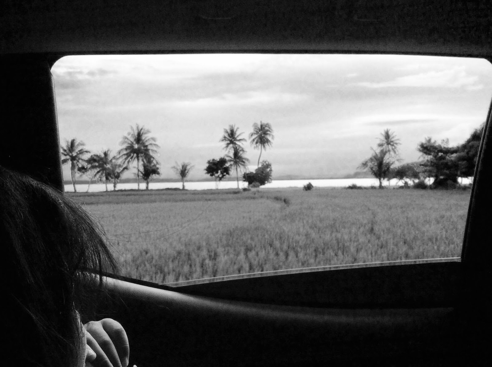
Image Negatives. The images look amazing here. Though the converted nighttime image is close to being all-white, it still looks good in negative.

Dimmed Images. The effect of dimming the images made them look like nighttime images.

Brightened Images. The brightened images made them look like some fog was all over the camera causing the effect. It's more noticeable on the daytime photo.

The next task was to get the gray images of the same photos, then get their histograms.

This one has many white and gray levels.

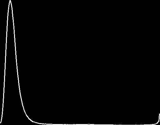
Since the original image was a nighttime image, most of the colors were dark, thus there are more black levels and grayish-black levels.

While the original images was a day time images, due to binarization, there were more gray levels than white levels.

This one had more black levels compared to gray and white levels.

Exercise 11 - Chroma Keying

https://www.youtube.com/watch?v=xPe6O__Iq5o&t=3s

For this exercise, we had to emulate an Opening Theme from an anime series. Fortunately for us, we got the Opening Theme of Slam Dunk. While it was embarrassing to be doing such things, it was for the academic value. It went well, to be honest... except for the rendering part. The code was easily made, but we had difficulties in rendering the video, since it took so much time and it used up so much ram that I had to restart my laptop after a video has rendered. Also, my laptop would really hang when 480p and better videos were rendered, so we had to stick to 360p instead. While the video output was embarrassing to watch, I could say we did a good job on this exercise.

Exercise 10 - Color Tracking

The exercise is now about Color Tracking, and what we were required to do is to create a triangle on the middle, then get the mean of the color value. Once the mean has been retrieved, we use it as a scalar value and use it as the color of the line drawing. We were given a sample code already, so the next step was just to modify the color of the line.

Exercise 9 - Background Subtraction

This exercise involved taking out the background and leaving the foreground of the video. Our lab instructor had already provided the code, but the output of the said code was a black foreground. Our exercise involved producing the actual foreground, and on a video output file.

While we weren't able to finish the exer, we did understand how background subtraction on videos work. The video will have to be spliced to frames, then each frame would be studied for a possible background, then the studied background is subtracted to all frames, then the processed frames are made to a video again.

Exercise 8 - Color Tracking

This exercise was about false coloring, and we were required to apply our own color scale on the sea part of the provided images. It was fairly easy, as we used the inRange() function for identifying the blue waters part of the images.

Exercise 7 - OCR Part 1

For this exercise, we were made to produce 20 images of handwritten numbers, with one number per image, then and another 20 images of computer-made numbers, then using our own implementation of OCR, we must be able to study and learn the features of the computer-made numbers, then identify the numbers written on the handwritten number images. The determinant for identifying the numbers was using a Euclidean distance formula. We used Area, Height, and Width for the exercise.

While our exercise worked without much error, we were only able to identify 25% of the images. It was still good, despite that we already had used 3 features for the exercise. Some identifications were really far (like 3 identified as 7) and some are close (like 9 identified as 0).

Exercise 6 - Erosion-Dilation

This exercise is about using image erosion and image dilation techniques in order to fix up some sample student evaluation forms, then tally the results. What we did was binarize the image first through thresholding, then experiment on using the erode and dilate to emphasize the marks that were shaded. We mapped the individual coordinates first, then tally the results and record them on a text file.

Exercise 5 - Blobs

In this exercise, we had to (1) identify the coins and compute for the total amount of the coins on the photo provided, and then we had to (2) identify the images on another photo.
While we did not follow the instructions for labeling the coins and images (LOL), we were able to identify the coins present on the first photo, as well as the objects on the second photo. We had a bit of problem when it came to OpenCV versions, as some functions work differently on some versions, but it wasn't that big of a problem in regards to doing the exercise.

Original coins image.

 Labeled coins, they should be labeled using bounding boxes.

 Original objects image

Labeled image

Exercise 3

The exercise that week was about Filtering images. The exercise required us to make a medianBlur filtering function. The exercise was rather easy, however my partner and I had some troubles.

First off, the function we made only catered to kernels with only 1 as their values. The function wouldn't work well on kernels with different cell values. Second, because of the first problem, we couldn't test other kernels such as the Gaussian Kernel.

While we both learned how filtering works, it was such a shame that we weren't able to do the exercise correctly.

Exercise 4 was rather a mix of easy and hard, unlike the other exercises. The exercise was all about binarization and edge detection. Binarization is a process of turning the photo foreground to black, then the background would be white, or vice versa, given a threshold. Edge Detection simply means detecting the edges or outlines of the foreground of the photo.

Now why did I thought it was a mix of easy and hard? That's because the difficulty of these two processes depends on the photo one is working with. For example, in the Binarization part, we found the quote.jpg and magazin1.jpg easier to binarize, while magazin2.jpg was harder to binarize. My partner and I used brute force to get rid of the annoying background so it would be easier to make the text appear.

Original quote.jpg.

Binarized quote.jpg where the the letters of the image are all in black.

Original magazin1.jpg.

Binarized magazin1.jpg.

Original magazin2.jpg.

Binarized magazin2.jpg. Notice how the photo is still not clean and still has the noise from the original photo.

As for the Edge Detection part, the photo was really hard to work on with, since one part looked illuminated while the other didn't. While I was able to (somehow) get the edges, the algorithm we did may not be correct as we still used brute force to binarize the photo.

Original source.png.

Binarized source.png.

While I understood the purpose of Binarization, I didn't appreciate the Edge Detection much, since it invloved a lot of steps compared to Binarization. I still understood the two concepts nonetheless. Hopefully I would get to appreciate Edge Detection when we get to the later exercises.

Exercise 1

I never really thought image processing would involve so much Math and everything. Of course I expected Math since this is a CMSC course, but I didn't anticipate the first exercise would have a formula for it to be solved.
The first exercise involved two photos of teachers, A and B. We have to manipulate teacher A and turn it to teacher B by using a certain formula that will transform all pixels until A transforms to B. Pretty cool if you'd ask me, but formulating an algorithm is a bit tricky, in my opinion. When I finally thought I got how to solve the exercise, it was already time...
While what my partner and I did on the exercise didn't came out right, at least we now know that image transformations are performed and manipulated using formulas, and each formula gives the image a different transformation.